Probably Approximately Correct
Питання Валіанта (1984)
Леслі Валіант поставив на перший погляд просте запитання: що означає, коли машина вчиться? Не «чи може вона запам’ятовувати?» і не «чи може вона передбачати ідеально?». Натомість: чи може вона вчитися приблизно добре, з високою ймовірністю, з обмеженої вибірки та за поліноміальний час?
Саме це формулювання принесло йому премію Тюрінга 2010 року та заклало основи обчислювальної теорії навчання.
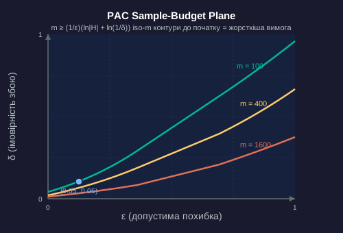
Два регулятори
ε (епсилон) — допустима похибка. Приблизно правильне означає, що похибка ≤ ε. Менше ε = жорсткіше навчання.
δ (дельта) — параметр довіри. Ймовірнісно означає, що ймовірність успіху ≥ 1 − δ. Менше δ = вища потрібна впевненість.
Визначення
Клас концепцій C вважається PAC-навчальним, якщо існує алгоритм, який для будь-якого розподілу даних D та будь-якої цільової концепції c ∈ C, отримавши m прикладів, вибраних з D та позначених c, повертає гіпотезу h, що задовольняє:
P[error(h) ≤ ε] ≥ 1 − δ
де m є поліноміальним за 1/ε, 1/δ та розміром концепції.
In Ukrainian: годувати достатньою кількістю прикладів — і модель достатньо часто наближається до потрібного результату, причому «достатньо» не зростає експоненційно.
Об’єм вибірки для скінченних просторів гіпотез
Якщо простір гіпотез H містить скінченну кількість кандидатів, класичний аналіз дає:
m ≥ (1/ε)(ln|H| + ln(1/δ))
Інтерпретуйте цю формулу як бюджет. Зменшення ε вдвічі подвоює потрібну кількість зразків. Зменшення δ додає константу. Збільшення |H| вдвічі додає лише ln(2) зразків — логарифмічне зростання, приємно стримане.
Визначення розміру вибірки для гіпотезного класу
Спам-фільтр обирає серед |H| = 1 000 000 кандидатних наборів правил. Ми хочемо, щоб помилка ε ≤ 0,05 з довірою 1 − δ = 0,99 (тобто δ = 0,01).
Розбиття та VC-вимір
Коли простори гіпотез стають нескінченними
Оцінка m ≥ (1/ε)(ln|H| + ln(1/δ)) перестає працювати, коли |H| = ∞. Більшість корисних класів гіпотез (лінійні класифікатори в ℝᵈ, дерева рішень, нейронні мережі) містять нескінченно багато кандидатів. Вапник і Червоненкіс розв’язали цю проблему близько 1971 року, запропонувавши складнішу міру складності: VC-розмір.

Шаттерінг
Клас гіпотез H шаттерує набір із n точок, якщо H здатен реалізувати будь-яке можливе маркування цих n точок (усі 2ⁿ дихотомії). Лінійні класифікатори в ℝ² шаттерують будь-які 3 точки в загальному положенні: для кожного з 8 можливих +/- маркувань цих 3 точок існує пряма, яка правильно їх розділяє.
Але лінійні класифікатори в ℝ² не можуть розбити 4 точки, розташовані в конфігурації XOR. Жодна пряма лінія не відокремлює діагональну пару від антидіагональної пари.
VC-розмірність
VC(H) = найбільше n, для якого H розбиває деяку множину з n точок. Для лінійних класифікаторів у 2D: VC = 3. Для осесиметричних прямокутників у 2D: VC = 4. Для нейронних мереж із W вагами: VC ≤ O(W² log W) (Bartlett & Anthony 1999).
Об’єм вибірки з VC-розмірністю
Замініть ln|H| у нашій PAC-межі на VC-розмірність d:
m = O((d/ε) log(1/ε) + (1/ε) log(1/δ))
VC-розмірність виступає як наша «ефективна складність» нескінченного класу. Гіпотезний клас із низькою VC-розмірністю узагальнюється з невеликої кількості зразків; клас із високою VC-розмірністю потребує більше даних.
VC-розмірність як ефективна кількість гіпотез
Нейронна мережа має W = 10⁹ ваг. Згідно з межею Бартлетта-Ентоні, VC ≤ O(W² log W). Приблизно VC ≈ W² log₂ W.
Відмова від реалізованості, апостеріорні розподіли над гіпотезами
Дві важливі узагальнення
Класичний PAC припускає, що цільова концепція c знаходиться всередині нашого класу гіпотез H. Реальні дані містять шум, помилкові мітки та концепції, які наш клас не може представити. Два розширення це враховують.
Агностичний PAC
Відмовляємося від припущення, що c ∈ H. Тепер конкуруємо з нашою найкращою в класі гіпотезою h* = argmin_{h ∈ H} risk(h). Змінюється форма межі: замість наближення до ідеального результату ми наближаємося до найкращого можливого в межах H.
Агностична межа: P[risk(h) ≤ risk(h*) + ε] ≥ 1 − δ зі складністю вибірки m = O(1/ε² × (VC(H) + log(1/δ))). Зверніть увагу на ε² замість ε у знаменнику: агностичне навчання потребує більше прикладів для тієї ж точності.
PAC-Баєс (McAllester 1999)
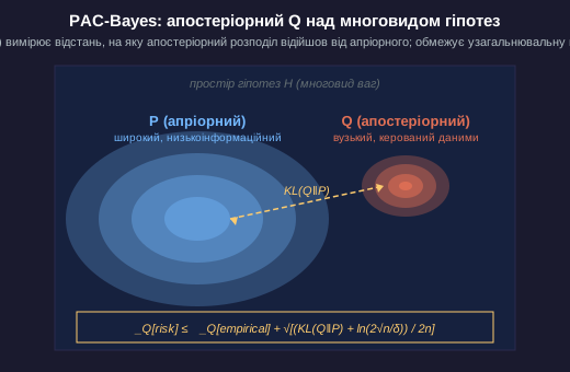
Переходимо від вибору однієї гіпотези до вибору розподілу над гіпотезами. Починаємо з апріорного розподілу P. Спостерігаємо дані. Отримуємо апостеріорний розподіл Q. Межі PAC-Баєс дають очікуваний ризик за Q:
𝔼_{h~Q}[risk(h)] ≤ 𝔼_{h~Q}[empirical_risk(h)] + √[(KL(Q‖P) + ln(2√n/δ)) / 2n]
KL(Q‖P) показує, наскільки наша апостеріорна розподіл змістився відносно апріорного. Дві інтерпретації:
1. Погляд через стиснення. Апостеріорний розподіл, близький до апріорного (малий KL), добре узагальнює — мала інформаційна вартість = малий розрив узагальнення.
2. Байєсівський погляд. Сильний апріор + слабке оновлення за даними = жорстка межа; слабкий апріор + сильне оновлення за даними = менш жорстка межа.
Чому PAC-Bayes важливий. Емпіричні PAC-Bayes межі (Catoni 2007, Dziugaite & Roy 2017) дають чисельно значущі гарантії узагальнення для реальних нейронних мереж, де класичні PAC-межі стають порожніми. Вони залишаються нашим найточнішим теоретичним інструментом для аналізу узагальнення в перепараметризованих моделях.
Reading a PAC-Bayes Bound
Припустимо, ми навчаємо мережу на n = 50 000 розмічених прикладів. Після навчання наша апостеріорна Q над вагами має KL(Q‖P) = 200 нат відносно гаусового апріорного P. Емпіричний ризик за Q становить 0.10. Встановіть δ = 0.05.
Перепараметризація та подвійний спуск
Класична теорія PAC передбачає катастрофу
Класична теорія PAC передбачає: більше параметрів, ніж прикладів = катастрофічне перенавчання. Ідеальне запам’ятовування тренувальних даних і випадкове узагальнення на тестових. Межа VC передбачає запам’ятовування без навчання.
Сучасні нейронні мережі зазвичай мають у 10–1000 разів більше параметрів, ніж прикладів для навчання, і все одно добре узагальнюються. За класичною теорією цього не мало б відбуватися. Але це відбувається.
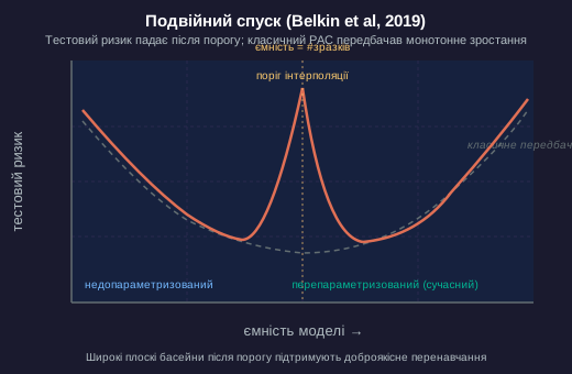
U-подібна крива, якій нас вчили
Класична дилема «зсув–розкид»: зі зростанням ємності моделі помилка на тренуванні монотонно зменшується; помилка на тесті спочатку падає (зменшується underfit), досягає мінімуму, а потім зростає (overfit). U-подібна крива, передбачена теорією VC.
Що відбувається насправді — Подвійний спуск
Belkin et al (2019) показали, що помилка на тесті дотримується класичної U-подібної кривої до порогу інтерполяції (ємність = кількість зразків), а потім знову ПАДАЄ після цього порогу. Масово перепараметризовані моделі узагальнюються краще, ніж моделі «достатньої» ємності.
Чому класична PAC-теорія це не пояснює
1. Припущення про незалежність від розподілу занадто песимістичне. Реальні дані мають структуру (низька внутрішня розмірність, геометрія многовиду). PAC-границі справедливі для найгіршого випадку розподілу; реальні розподіли використовують структуру, яку також експлуатує SGD.
2. Неявна регуляризація. SGD на перепараметризованих мережах знаходить інтерполюючі розв’язки з мінімальною нормою або мінімальною складністю, а не довільні. Класична теорія припускає найгірший емпіричний мінімізатор ризику; реальні алгоритми обирають «доброзичливі» розв’язки.
3. Неправильне визначення класу гіпотез. Ефективний клас гіпотез, який досліджує SGD, значно менший за номінальний простір ваг. Постеріори PAC-Bayes це враховують; VC-розмірність — ні.
Сучасні теоретичні дослідження (Bartlett, Long, Lugosi, Tsigler 2020 щодо доброякісного перенавчання; Nakkiran et al 2020 щодо подвійного спуску) формують пост-PAC теорію узагальнення, яка враховує режим перепараметризації.
Діагностика невдачі класичної PAC
Дослідницька група навчає мережу з 1 мільярдом параметрів на 100 000 розмічених прикладів. Класична PAC передбачає порожні межі. Емпірично тестова точність досягає 95 %.
Kaplan, Chinchilla та Розмір Автоматизованого Загального Інтелекту
Від меж до емпіричних законів масштабування
Класичний PAC теоретично передбачає розмір набору даних і дає порожні результати. Емпіричні закони масштабування передбачають розмір набору даних на основі спостережень і реально працюють. Вони замінили PAC як практичний інструмент визначення розміру для великих моделей.
Kaplan та ін. (2020)
Втрати підпорядковуються степеневому закону залежно від кількості параметрів N, токенів у наборі даних D та обчислювальних ресурсів C:
L(N) ≈ (Nc/N)^αN L(D) ≈ (Dc/D)^αD L(C) ≈ (Cc/C)^αC
Подвоєння кількості параметрів зменшує втрати на фіксований мультиплікативний коефіцієнт. Подвоєння обсягу даних зменшує втрати на інший фіксований коефіцієнт. Ці показники степеня (αN, αD, αC) вимірюють і прогнозують поведінку на передовій межі на багатьох порядках величини.
Hoffmann et al 2022 (Chinchilla)
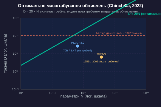
Chinchilla показала, що експоненти Каплана надмірно зважували параметри відносно даних. Оптимальне за обчисленнями тренування потребує приблизно 20 токенів на параметр:
D_opt ≈ 20 × N
GPT-3 (175 млрд параметрів) навчали на ~300 млрд токенів — значно недотренована модель за підрахунками Chinchilla. Обчислювально-оптимальна модель на 175 млрд параметрів потребує ~3,5 трильйона токенів.
The Data Wall
Масштабування кількості параметрів вимагає пропорційного масштабування кількості токенів. Публічний веб-краулінг дає ~10¹³ корисних токенів. Гіпотетичний автоматизований загальний інтелект на 10¹⁵ параметрів потребував би ~2×10¹⁶ токенів — на три порядки більше, ніж доступно у веб-даних.
Це наша data wall. Scaling laws передбачають, що ми зіткнемося з нестачею корпусу задовго до нестачі обчислювальних ресурсів. Синтетичні дані, мультимодальні корпуси (відео, аудіо, сенсорні потоки) та RL-from-environment спрямовані на подолання цієї межі.
Класична теорія PAC (неправильно) стверджувала, що нам потрібно 10²¹ зразків. Scaling laws (калібровані до реальності) показують, що потрібно 2×10¹⁶. Обидва числа перевищують доступний текст. Сучасні frontier-дослідження зосереджені на подоланні цього розриву.
Оцінювання корпусу для Automated General Intelligence
Припустимо, що frontier-лабораторія пропонує модель на 10¹⁴ параметрів і стверджує, що вона досягне automated general intelligence. Ми хочемо визначити розмір її навчального корпусу за правилом Chinchilla.
Від теоретичних меж до продакшн-вимірювань [BLOCK_TYPE production_audit/audit_content]
Припиніть обчислювати межі; почніть їх вимірювати
[BLOCK_TYPE production_audit/audit_content]Класичні PAC-межі є порожніми. PAC-Bayes межі стають щільними лише за припущень, які важко перевірити. Практична альтернатива: вимірюйте ε емпірично на вашому реальному розподілі та оновлюйте його під час роботи системи. [BLOCK_TYPE production_audit/audit_content]
Ідея 1 — Зробити покриття як емпіричний PAC
Ціль make coverage запускає N відкладених питань через вашу систему запитів і вимірює два показники:
- cache_hit_rate — частка, коли система знайшла відому відповідь
- i_dont_know_rate — частка, коли система чесно відмовилася відповідати
Кожне вимірювання = випробування Бернуллі. Зі спостережуваних частот обчислюємо інтервал Вілсона для справжньої частоти. Приклад: N = 1000 запитів, i_dont_know_rate = 0.20 → 95% ДІ ≈ [0.177, 0.226]. Верхня межа 0.226 функціонує точно як PAC ε при δ = 0.05, отримана з реальних даних на реальному розподілі, а не з найгіршого теоретичного аналізу.
Класична PAC-термінологія застосовується (ε, δ, довірча ймовірність). Інший математичний апарат (біноміальна концентрація замість VC-теорії). Результат точніший, бо реальні розподіли мають структуру, яку можна використовувати.
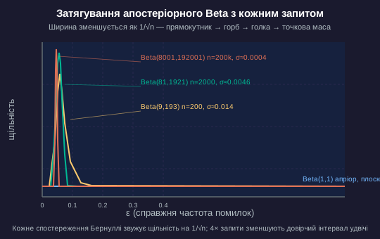
Ідея 2 — PAC-Байєсівський аудит через події фальсифікації
Кожну фальсифікацію (коли відповідь системи явно неправильна) розглядаємо як свідчення, що оновлює апостеріорний розподіл справжньої частоти помилок ε:
1. Апріор: ε ~ Beta(α₀, β₀). Обираємо слабкий апріор, наприклад Beta(1, 1) = рівномірний.
2. Кожен запит дає результат за розподілом Бернуллі: фальсифікований (1) або не фальсифікований (0).
3. Апостеріорний розподіл після k фальсифікацій у n запитах: Beta(α₀ + k, β₀ + n − k).
4. Апостеріорне середнє: (α₀ + k) / (α₀ + β₀ + n) → емпірична частота фальсифікацій при n → ∞.
5. 95% довірчий інтервал для ε звужується як 1/√n.
Що це нам дає
- Реальна оцінка ε₀ з фактичного розгортання, а не з теорії найгіршого випадку
- Anytime-valid alarm: коли задній довірчий інтервал перетинає поріг контракту, сповістити когось
- Монотонна довірливість: більше спостережених запитів → вужчий ДІ → сильніша гарантія
Споріднені методи: конформне передбачення з онлайн-перекалібруванням (Vovk), послідовні ймовірнісні відношення (Wald), онлайн PAC-Bayes (Haddouche & Guedj 2022). Одна родина, різні математичні апарати.
Обчислення апостеріорного Beta-розподілу для фальсифікацій
Наша команда проводить аудит покриття на продакшн-системі запитів. Апріорна ймовірність істинної частки помилок ε: Beta(1, 1) (рівномірний). Після 200 відкладених запитів ми зафіксували 8 фальсифікацій.