التعلم الاحتمالي التقريبي
سؤال فاليانت (1984)
طرح ليزلي فاليانت سؤالاً بسيطاً ظاهرياً: ماذا يعني أن تتعلم الآلة؟ ليس "هل تستطيع الحفظ؟" وليس "هل تستطيع التنبؤ بدقة كاملة؟" بل: هل تستطيع التعلم بشكل تقريبي جيد، باحتمالية عالية، من عينة محدودة، في زمن متعدد الحدود؟
هذا الإطار حصل به على جائزة تورينج عام 2010 وأسس نظرية التعلم الحاسوبي.
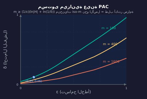
مقبضان
ε (إبسيلون) — درجة تحمّل الخطأ. التعلم التقريبي الصحيح يعني أن الخطأ ≤ ε. كلما صغر ε زادت صرامة التعلم.
δ (دلتا) — معامل الثقة. "ربما" تعني أن احتمال النجاح ≥ 1 − δ. كلما صغر δ زادت الثقة المطلوبة.
التعريف
تُعد فئة المفاهيم C قابلة للتعلم بطريقة PAC إذا وُجدت خوارزمية بحيث، لأي توزيع بيانات D وأي مفهوم مستهدف c ∈ C، وعند إعطاء m عينة مسحوبة من D ومُصنَّفة بواسطة c، تُرجع الخوارزمية فرضية h تحقق:
P[error(h) ≤ ε] ≥ 1 − δ
حيث يكون m متعدد الحدود في 1/ε، 1/δ، وحجم المفهوم.
في الإنجليزية: أعطِه أمثلة كافية وسيصل إلى نتيجة قريبة بما يكفي في أغلب الأحيان، و"الكفاية" لا تنفجر أسّيًا.
تعقيد العينة لفضاءات الفرضيات المحدودة
إذا كان فضاء الفرضيات H يحتوي على عدد محدود من الفرضيات المرشحة، فإن التحليل الكلاسيكي يعطي:
m ≥ (1/ε)(ln|H| + ln(1/δ))
اقرأ هذه الصيغة كميزانية. خفض ε إلى النصف يضاعف عدد العينات المطلوبة. خفض δ إلى النصف يضيف ثابتًا. مضاعفة |H| تضيف ln(2) عينة — نمو لوغاريتمي، وهو نمو جميل ومسيطر عليه.
تحجيم عينة لفئة فرضيات
يختار مرشح البريد العشوائي من بين |H| = 1,000,000 مجموعة قواعد مرشحة. نريد خطأ ε ≤ 0.05 مع ثقة 1 − δ = 0.99 (أي δ = 0.01).
التحطيم وبُعد VC
عندما تصبح فضاءات الفرضيات لا نهائية
تنهار المتباينة m ≥ (1/ε)(ln|H| + ln(1/δ)) عندما يكون |H| = ∞. معظم فئات الفرضيات المفيدة (المصنفات الخطية في ℝᵈ، أشجار القرار، الشبكات العصبية) تحتوي على عدد لا نهائي من المرشحين. حل فابنيك وتشيرفونينكيس هذه المشكلة حوالي عام 1971 بمقياس أغنى للتعقيد: بُعد VC.

التحطيم (Shattering)
تقول فئة الفرضيات H إنها تحطم مجموعة من n نقاط إذا استطاعت H إنتاج كل تسمية ممكنة لهذه النقاط (جميع التقسيمات الثنائية البالغ عددها 2ⁿ). تستطيع المصنفات الخطية في ℝ² تحطيم أي 3 نقاط في وضع عام: فمن أجل كل واحدة من التسميات الثمانية الممكنة (+/−) لهذه النقاط الثلاث، يوجد خط يفصلها بشكل صحيح.
لكن المصنفات الخطية في ℝ² لا تستطيع تحطيم 4 نقاط مرتبة في تكوين XOR. لا يوجد خط مستقيم يفصل الزوج القطري عن الزوج المضاد للقطري.
البعد VC
VC(H) = أكبر قيمة n بحيث تستطيع H تحطيم مجموعة من n نقطة. بالنسبة للمصنفات الخطية ثنائية الأبعاد: VC = 3. بالنسبة للمستطيلات المحاذية للمحاور في 2D: VC = 4. بالنسبة للشبكات العصبية التي تحتوي على W أوزان: VC ≤ O(W² log W) (Bartlett & Anthony 1999).
تعقيد العينة باستخدام بعد VC
استبدل ln|H| في حد PAC لدينا ببعد VC المسمى d:
m = O((d/ε) log(1/ε) + (1/ε) log(1/δ))
يعمل بُعد VC كـ"التعقيد الفعّال" لصفٍ لا نهائي. فصف الفرضيات ذو بُعد VC منخفض يعمّم من عيّنات قليلة، بينما يحتاج الصف ذو بُعد VC مرتفع إلى المزيد من البيانات.
بُعد VC كعدد فرضيات فعّال
تحتوي شبكة عصبية على W = 10⁹ وزن. وفقًا لحدّ Bartlett-Anthony، فإن VC ≤ O(W² log W). نقرّب VC ≈ W² log₂ W.
إسقاط التحقق، التوزيعات اللاحقة على الفرضيات
تعميمان مهمان
يفترض PAC الكلاسيكي أن المفهوم المستهدف c يقع داخل صف الفرضيات H. تحمل البيانات الحقيقية ضوضاء وتسميات خاطئة ومفاهيم لا يستطيع صفنا تمثيلها. يعالج امتدادان هذا الأمر.
PAC اللامعرفي
نتخلى عن افتراض أن c ∈ H. الآن ننافس أفضل فرضية لدينا h* = argmin_{h ∈ H} risk(h). يتغير شكل الحد: بدلاً من الاقتراب من الكمال، نقترب من الأفضل الممكن داخل H.
الحد اللامعرفي: P[risk(h) ≤ risk(h*) + ε] ≥ 1 − δ مع تعقيد العينة m = O(1/ε² × (VC(H) + log(1/δ))). لاحظ ε² بدلاً من ε في المقام: التعلم اللامعرفي يحتاج إلى المزيد من العينات لنفس الدقة.
PAC-بايز (ماك أليستر 1999)
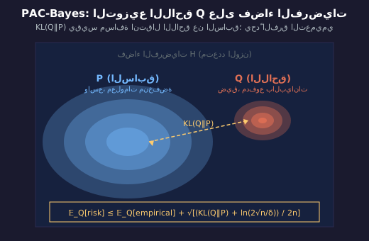
ننتقل من اختيار فرضية واحدة إلى اختيار توزيع على الفرضيات. نبدأ بتوزيع مسبق P. نلاحظ البيانات. نستنتج التوزيع اللاحق Q. حدود PAC-بايز تقيس المخاطرة المتوقعة تحت Q:
𝔼_{h~Q}[risk(h)] ≤ 𝔼_{h~Q}[empirical_risk(h)] + √[(KL(Q‖P) + ln(2√n/δ)) / 2n]
KL(Q‖P) يقيس مدى ابتعاد التوزيع اللاحق (posterior) عن التوزيع السابق (prior). هناك تفسيران:
1. منظور الضغط (Compression view). التوزيع اللاحق القريب من التوزيع السابق (KL صغير) يعمم جيدًا — تكلفة معلوماتية صغيرة = فجوة تعميم صغيرة.
2. المنظور البيزي (Bayesian view). أولوية قوية + تحديث بيانات ضعيف = حد محكم؛ أولوية ضعيفة + تحديث بيانات كبير = حد أوسع.
لماذا يهم PAC-Bayes. توفر حدود PAC-Bayes التجريبية (Catoni 2007, Dziugaite & Roy 2017) ضمانات تعميم عددية ذات معنى للشبكات العصبية الحقيقية، حيث تكون حدود PAC الكلاسيكية فارغة. وهي لا تزال أقوى أداة نظرية لدينا لفهم التعميم في النماذج ذات المعاملات الزائدة.
قراءة حد PAC-Bayes
افترض أننا درّبنا شبكة على n = 50,000 مثالاً مصنفاً. بعد التدريب، يكون للتوزيع اللاحق Q على الأوزان KL(Q‖P) = 200 نات بالنسبة للتوزيع السابق الغاوسي P. يبلغ الخطر التجريبي تحت Q 0.10. اضبط δ = 0.05.
الإفراط في البارامترات والهبوط المزدوج
توقّع الكارثة في PAC الكلاسيكي
توقّع PAC الكلاسيكي: عدد المعاملات أكبر من عدد العينات = فرط تكيّف كارثي. تعلّم مثالي على بيانات التدريب، وتعميم عشوائي على بيانات الاختبار. يتنبأ حد VC بالحفظ دون تعلّم.
الشبكات العصبية الحديثة غالبًا ما تحتوي على 10× إلى 1000× معاملات أكثر من عينات التدريب، ومع ذلك تُعمّم. هذا لا يجب أن يحدث وفق النظرية الكلاسيكية. لكنه يحدث على أي حال.
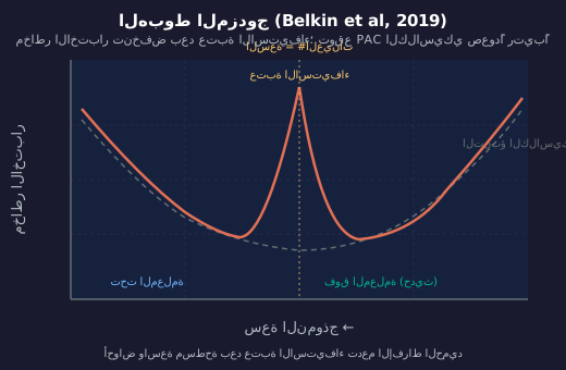
منحنى U الذي تعلّمناه
التحيز والتباين الكلاسيكي: مع زيادة سعة النموذج، ينخفض خطأ التدريب بشكل رتيب؛ أما خطأ الاختبار فيبدأ بالانخفاض (بسبب تقليل الـ underfit)، ثم يصل إلى الحد الأدنى، ثم يرتفع (بسبب الـ overfit). منحنى U المتوقع من نظرية VC.
ما يحدث فعليًا — النزول المزدوج
أظهر بيلكين وآخرون (2019) أن خطأ الاختبار يتبع منحنى U الكلاسيكي حتى عتبة الاستيفاء (السعة = عدد العينات)، ثم ينخفض مرة أخرى بعد تجاوز هذه العتبة. النماذج ذات المعاملات الزائدة بشكل كبير تعمم بشكل أفضل من النماذج الكبيرة بما يكفي فقط.
لماذا يفوت PAC الكلاسيكي هذا
1. افتراض الخلو من التوزيع متشائم جدًا. البيانات الحقيقية تحتوي على بنية (بعد جوهري منخفض، هندسة متعددة الشعب). حدود PAC تنطبق على أسوأ التوزيعات؛ أما التوزيعات الحقيقية فتستغل البنية التي يستغلها أيضًا SGD.
2. التنظيم الضمني. يجد SGD على الشبكات المفرطة البارامترات حلولاً ذات الحد الأدنى من المعيار أو الحد الأدنى من التعقيد، وليس حلولاً عشوائية. تفترض النظرية الكلاسيكية أسوأ حالة لمُقلل المخاطر التجريبية؛ بينما تختار الخوارزميات الحقيقية حلولاً حميدة. [BLOCK_TYPE SECTION/STEP]
3. تعريف فئة الفرضيات خاطئ. فئة الفرضيات الفعالة التي يستكشفها SGD أصغر بكثير من فضاء الأوزان الاسمي. تلتقط خلفيات PAC-Bayes هذا؛ بينما لا يلتقطه بُعد VC. [BLOCK_TYPE SECTION/STEP]
[BLOCK_TYPE SECTION/STEP]
تعمل الأبحاث النظرية الحديثة (Bartlett, Long, Lugosi, Tsigler 2020 حول الإفراط الحميد؛ Nakkiran et al 2020 حول النزول المزدوج) على بناء نظرية تعميم ما بعد PAC تأخذ في الاعتبار نظامنا المفرط البارامترات.
تشخيص فشل PAC الكلاسيكي [BLOCK_TYPE SECTION/STEP]
تقوم فريق بحثي بتدريب شبكة تحتوي على مليار بارامتر على 100,000 مثال مُعَلَّم. تتنبأ PAC الكلاسيكية بحدود فارغة. تجريبياً، تصل دقة الاختبار إلى 95%.
كابلان، تشينشيلا، وحجم الذكاء العام الآلي
من الحدود إلى قوانين التوسع التجريبية
يتنبأ PAC الكلاسيكي بحجم مجموعة البيانات نظريًا ويكون فارغًا. قوانين التوسع التجريبية تتنبأ بحجم مجموعة البيانات من الملاحظة وتعمل فعليًا. لقد حلت محل PAC كأداة عملية لتحديد حجم النماذج الكبيرة.
كابلان وآخرون (2020)
يتبع الفقدان قانون قوة في المعاملات N، ورموز مجموعة البيانات D، والحوسبة C:
L(N) ≈ (Nc/N)^αN L(D) ≈ (Dc/D)^αD L(C) ≈ (Cc/C)^αC
مضاعفة المعاملات تقلل الفقدان بعامل مضاعف ثابت. مضاعفة البيانات تقلل الفقدان بعامل ثابت آخر. تقيس هذه الأسس (αN, αD, αC) وتتنبأ بسلوك الحدود عبر العديد من مراتب الحجم.
هوفمان وآخرون 2022 (Chinchilla)
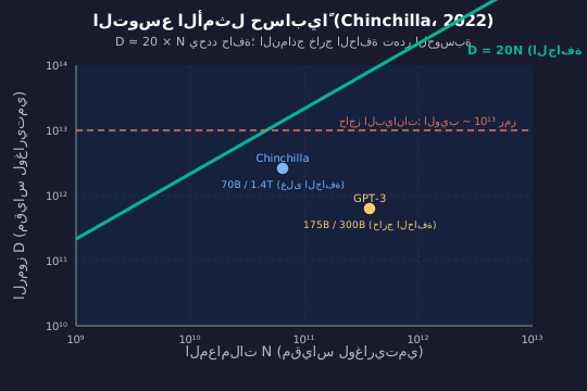
أظهرت Chinchilla أن معاملات كابلان أعطت وزناً زائداً للمعاملات مقارنة بالبيانات. يتطلب التدريب الأمثل حسابياً حوالي 20 توكناً لكل معامل:
D_opt ≈ 20 × N
تم تدريب GPT-3 (175B معامل) على حوالي 300B توكناً — وهو تدريب ناقص جداً وفقاً لحسابات Chinchilla. يحتاج نموذج 175B معامل مثالي حسابياً إلى حوالي 3.5 تريليون توكناً.
جدار البيانات
يتطلب توسيع عدد المعاملات توسيع عدد الرموز بشكل متناسب. يُنتج الزحف العام للويب حوالي 10¹³ رمزًا مفيدًا. وستحتاج ذكاء عام آلي افتراضي يحتوي على 10¹⁵ معامل إلى حوالي 2×10¹⁶ رمز — أي أكثر بثلاث مرات من البيانات المتاحة على الويب.
هذا هو جدار البيانات لدينا. تتنبأ قوانين التوسع بأننا سنواجه نقصًا في البيانات قبل أن نواجه نقصًا في الحوسبة. تهدف البيانات الاصطناعية، والمجموعات متعددة الوسائط (فيديو، صوت، تدفقات المستشعرات)، والتعلم المعزز من البيئة إلى تجاوز هذا الحاجز.
أخبرنا PAC الكلاسيكي (بشكل غير صحيح) أننا نحتاج إلى 10²¹ عينة. بينما تخبرنا قوانين التوسع (المعايرة مع الواقع) أننا نحتاج إلى 2×10¹⁶. وكلا الرقمين يتجاوزان النصوص المتاحة. يركز العمل الرائد اليوم على سد هذه الفجوة.
تقدير مجموعة بيانات الذكاء العام الآلي
افترض أن مختبرًا رائدًا يقترح نموذجًا يحتوي على 10¹⁴ معامل ويدّعي أنه سيصل إلى الذكاء العام الآلي. نريد تحديد حجم مجموعة بيانات التدريب الخاصة به وفقًا لقاعدة Chinchilla.
من الحدود النظرية إلى القياسات الإنتاجية
توقف عن حساب الحدود؛ ابدأ بقياسها
حدود PAC الكلاسيكية تصبح فارغة. حدود PAC-Bayes تكون محكمة لكن تحت افتراضات يصعب التحقق منها. البديل العملي: قِس ε تجريبيًا على التوزيع الحقيقي لديك وحدّثه مع تشغيل النظام.
الفكرة 1 — جعل التغطية كـ PAC تجريبي
هدف make coverage يُشغّل N سؤالاً محجوزاً عبر نظام الاستعلام الخاص بك ويقيس معدلين:
- cache_hit_rate — نسبة الحالات التي وجد فيها نظامك إجابة معروفة
- i_dont_know_rate — نسبة الحالات التي امتنع فيها نظامك بصراحة
كل قياس = تجربة برنولي. من الأعداد المرصودة، احسب فترة ثقة ويلسون للمعدل الحقيقي. مثال: N = 1000 استعلام، معدل i_dont_know_rate المرصود = 0.20 → 95% CI ≈ [0.177, 0.226]. الحد العلوي 0.226 يعمل تماماً كـ PAC ε عند δ = 0.05، مستمد من بيانات حقيقية على التوزيع الحقيقي بدلاً من التحليل النظري الأسوأ حالة.
تنطبق مفردات PAC الكلاسيكية (ε، δ، الثقة). آلية مختلفة (تركيز ثنائي الحد مقابل نظرية VC). نتيجة أدق لأن التوزيعات الحقيقية تحمل بنية يمكن استغلالها.
الفكرة 2 — تدقيق PAC-Bayes عبر أحداث التزييف
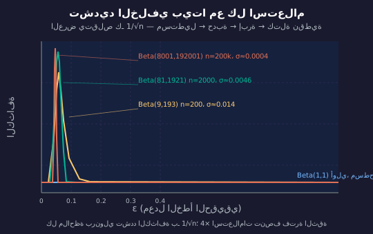
تعامل كل تزييف (إجابة النظام خاطئة بشكل مثبت) كدليل يحدّث التوزيع اللاحق لمعدل الخطأ الحقيقي ε:
1. التوزيع السابق: ε ~ Beta(α₀, β₀). اختر توزيعاً سابقاً ضعيفاً، مثل Beta(1, 1) = التوزيع المنتظم.
2. كل استعلام يُنتج نتيجة برنولي: مزيف (1) أو محتفظ به (0).
3. التوزيع اللاحق بعد k تزييفات في n استعلام: Beta(α₀ + k, β₀ + n − k).
4. متوسط التوزيع اللاحق: (α₀ + k) / (α₀ + β₀ + n) → معدل التزييف التجريبي عندما n → ∞.
5. فاصل المصداقية 95% على ε يضيق كـ 1/√n.
ما الذي يحققه لنا هذا
- تقدير ε₀ واقعي من النشر الفعلي، وليس نظرية الحالة الأسوأ
- إنذار صالح في أي وقت: عندما يتجاوز فاصل الثقة الخلفي عتبة العقد، يتم إشعار شخص ما
- ثقة رتيبة: كلما زادت الاستعلامات المرصودة → تضيّق فترة الثقة → ضمان أقوى
تقنيات مشابهة: التنبؤ المتوافق مع إعادة المعايرة عبر الإنترنت (Vovk)، اختبارات نسبة الاحتمال المتسلسلة (Wald)، PAC-Bayes عبر الإنترنت (Haddouche & Guedj 2022). نفس العائلة، آليات رياضية مختلفة.
حساب التوزيع الخلفي Beta للنتائج الخاطئة
يقوم فريقنا بتدقيق التغطية على نظام استعلام إنتاجي. التوزيع المسبق لمعدل الخطأ الحقيقي ε: Beta(1, 1) (موحد). بعد 200 استعلام محجوز لاحظنا 8 نتائج خاطئة.