बेल लैब्स, 1947
Richard Hamming 1946 में Bell Telephone Laboratories में शामिल हुए। वहां के relay computers केवल सप्ताह के दिनों में चलते थे, जब तकनीशियन त्रुटियों के बाद उन्हें पुनः आरंभ कर सकते थे। सप्ताहांत में, मशीनें जब कुछ गलत होता था तो बंद हो जाती थीं — नौकरियों को सोमवार तक कतार में छोड़ देती थीं।
हैमिंग क्रोधित थे। 'अगर मशीन एक त्रुटि का पता लगा सकती है,' उन्होंने सोचा, 'तो वह इसे खोज कर और सुधार क्यों नहीं सकती?' यह हताशा, binary arithmetic & parity checks के गहरे ज्ञान के साथ मिलकर, मंच तैयार करती है।
पहली अंतर्दृष्टि: आयताकार कोड
हैमिंग का पहला विचार: संदेश bits को एक m×n आयत में व्यवस्थित करना, हर row & हर column को एक parity check जोड़ना। एक single error ठीक एक विफल row check & एक विफल column check देता है। उनका प्रतिच्छेदन त्रुटि की स्थिति का नाम बताता है।
Redundancy ratio: (m+1)(n+1) / mn। Calculus बताता है कि एक वर्ग fixed message size के लिए इसे कम करता है। लेकिन जैसे m & n बढ़ते हैं, एक double error अधिक संभावित हो जाता है — एक engineering judgment बिना universal answer के।
आयताकार अतिरेक को कम करना
एक 4×4 आयत 16 message bits को 4 row checks & 4 column checks के साथ ले जाता है, साथ ही 1 corner parity bit = 16 message bits के लिए 9 check bits।
Redundancy ratio: (m+1)(n+1) / mn = 25/16 ≈ 1.56।
एक 10×10 आयत के लिए: 100 message bits, 121 कुल bits, redundancy ≈ 1.21।
सिंड्रोम एक बाइनरी संख्या के रूप में
rectangular code insight के कुछ हफ्तों बाद, हैमिंग New York की ओर New Jersey farmland में जा रहे थे, अपनी सफलताओं को mentally review कर रहे थे। Triangle code उसे आया — बेहतर redundancy। फिर cube। फिर 4-dimensional, 5-dimensional...
हर अतिरिक्त dimension ने redundancy में सुधार किया। n dimensions में side 2 का एक hypercube केवल n+1 parity checks को 2^n vertices के लिए उपयोग करता है। लेकिन क्या यह optimal था?
गिनती तर्क
n+1 parity bits एक syndrome देते हैं: एक (n+1)-bit binary number। वह syndrome को 2^n + 1 अलग-अलग outcomes की पहचान करने की आवश्यकता है: 2^n error positions में से प्रत्येक, साथ ही विशेष 'कोई त्रुटि नहीं' outcome।
2^(n+1) = 2·2^n — लगभग पर्याप्त। 2 के factor से बंद। हैमिंग ने समस्या को अलग रखा।
मुख्य अंतर्दृष्टि
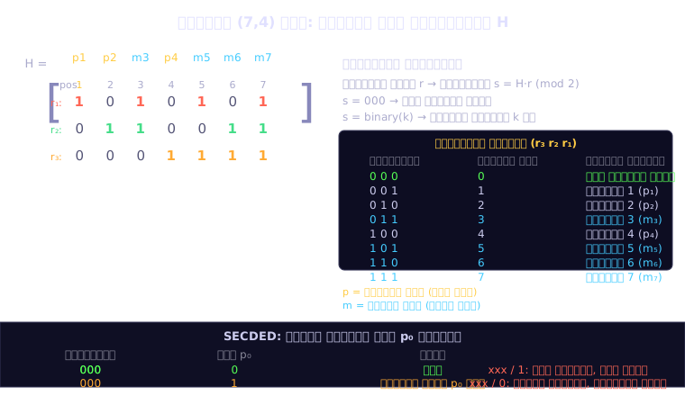
बाद में, हैमिंग एक नए विचार के साथ लौटे: syndrome को ही binary number के रूप में उपयोग करें जो त्रुटि position का नाम देता है। Position 1 = binary 001, position 2 = binary 010, position 3 = binary 011, आदि। सभी-zeros को 'कोई त्रुटि नहीं' के लिए reserve करें।
यह syndrome को parity checks के एक output से एक address में बदल देता है। Parity checks को ऐसा design करने के लिए किया जाता है कि जब कोई भी single bit flips तो ठीक सही address दें।
(7,4) कोड डिजाइन करना
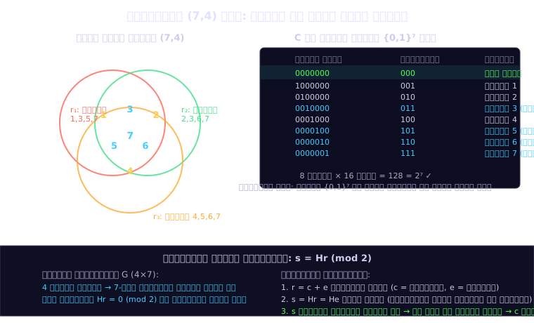
7-bit code के लिए (3 parity bits, 4 message bits), positions 1 से 7 binary में हैं: 001, 010, 011, 100, 101, 110, 111।
Parity check 1 positions को cover करता है जहां bit 0 = 1: positions 1, 3, 5, 7।
Parity check 2 positions को cover करता है जहां bit 1 = 1: positions 2, 3, 6, 7।
Parity check 3 positions को cover करता है जहां bit 2 = 1: positions 4, 5, 6, 7।
Parity bits power-of-2 positions पर कब्जा करती हैं: 1, 2, 4। Message bits बाकी पर कब्जा करती हैं: 3, 5, 6, 7।
अगर bit 6 flips होता है, parity checks 2 & 3 fail होते हैं (110 binary में = 6)। Syndrome पढ़ता है 110 = 6। Position 6 को flip करें। हो गया।
एकल त्रुटि सुधार, दोहरी त्रुटि पहचान
(7,4) Hamming code single errors को सुधारता है। लेकिन अगर दो bits flip होते हैं? अतिरिक्त सुरक्षा के बिना, decoder syndrome rule को apply करता है & codeword को गलत संदेश के लिए 'सुधारता है' — एक silent miscorrection।
SECDED: एक अतिरिक्त Parity Bit
पूरे codeword को cover करने वाला एक single parity bit p₀ जोड़ें (सभी 7 bits)। अब syndrome के पास 4 entries हैं: original 3 checks साथ ही p₀।
``
पुरानी syndrome  नई p₀  अर्थ
000           0       सही
000           1       केवल p₀ में त्रुटि
xxx           1       single error, पुरानी syndrome इसे नाम देती है
xxx           0       double error — इसे flag करें
``
चार cases exhaustive हैं। एक double error दो bits को flip करता है: पुरानी syndrome 000 नहीं पढ़ेगी (दोनों bits एक साथ इसके दो checks को corrupt करते हैं), लेकिन p₀ दो बार flip होता है और 0 पर वापस जाता है। Pattern xxx + 0 unmistakable है।
SECDED क्यों काम करता है
SECDED rule parity की modular structure को exploit करता है। Even parity के साथ, कोई भी single flip p₀ को बदलता है। कोई भी double flip p₀ को unchanged छोड़ता है। तो p₀ errors को modulo 2 गिनता है।
ज्यामितीय चित्र
हैमिंग एक अलग दिशा से एक ही जगह पर पहुंचे: analytic geometry। हर n-bit string को एक n-dimensional hypercube के एक vertex के रूप में represent करें। एक single bit flip एक point को एक edge-length एक axis के साथ move करता है। दो flips: दो edges। Metric है Hamming distance।
एक Hamming ball को radius t के साथ एक codeword c के चारों ओर define करें: c के t bit-flips के भीतर सभी points। Single-error correction के लिए, t = 1।
Single-error correction के लिए condition: distinct codewords की हर pair के चारों ओर radius 1 की balls overlap नहीं करनी चाहिए। अगर वे overlap करती हैं, तो overlap में एक received word दोनों codewords के लिए संबंधित हो सकता है & decoder fail।
यह directly minimum distance में translate करता है: दो radius 1 की balls overlap नहीं करती हैं अगर & केवल अगर codewords कम से कम 3 से अलग हों (d_min ≥ 3)।
(7,4) code d_min = 3 को achieve करता है। Hamming का bound: 2^7 / (1 + 7) = 16 = 2^4। ठीक 16 codewords। एक perfect code: radius 1 की 16 balls {0,1}^7 को कोई gaps या overlaps के साथ tile करती हैं।
इंजीनियरिंग निर्णय
हैमिंग explicit थे: error-correcting codes में engineering judgments होती हैं, pure mathematics नहीं।
संदेश length: longer messages अधिक efficient coding allow करते हैं (n message bits के लिए log n parity bits)। लेकिन longer messages भी अधिक noise accumulate करते हैं, एक double error के slipping through के जोखिम को एक false single correction के रूप में बढ़ाते हैं।
Level of correction vs. detection: एक error correction के लिए दो extra error detections को trading। Optimal split channel के noise characteristics पर निर्भर करता है।
Field maintenance value: जैसे equipment अधिक complex बन जाता है, field technicians हर failure को first principles से diagnose नहीं कर सकते। एक self-diagnosing system dramatically maintenance के लिए आवश्यक skill को reduce करता है। हैमिंग ने इसे सबसे महत्वपूर्ण benefits में से एक कहा, अक्सर raw reliability gain से अधिक महत्वपूर्ण।
शैली: भाग्य तैयार मन का पक्ष लेता है
हैमिंग ने अध्याय 12 को एक direct challenge के साथ बंद किया। उन्होंने discovery को three से six months के काम के रूप में describe किया, ज्यादातर odd moments में Bell Labs पर अपने main duties ले जाते हुए।
उन्होंने तीन चीजें identified कीं जो इसे possible बनाती थीं:
1. Preparation: parity checks, binary arithmetic, & group theory के साथ deep familiarity, समस्या appear होने से पहले।
2. Reviewing successes: habitually past solutions को replay करना उनकी style को internalize करने के लिए। Triangle code उसे एक commute पर rectangular code को mentally review करते हुए आया।
3. Not settling for 'looks good': उन्होंने एक बार अपनी उंगलियां burn कीं apparent optimality को accept करके। उन्होंने तब तक push किया जब तक वह code को best prove नहीं कर सकते।