Attention Plus MLP, Repeated
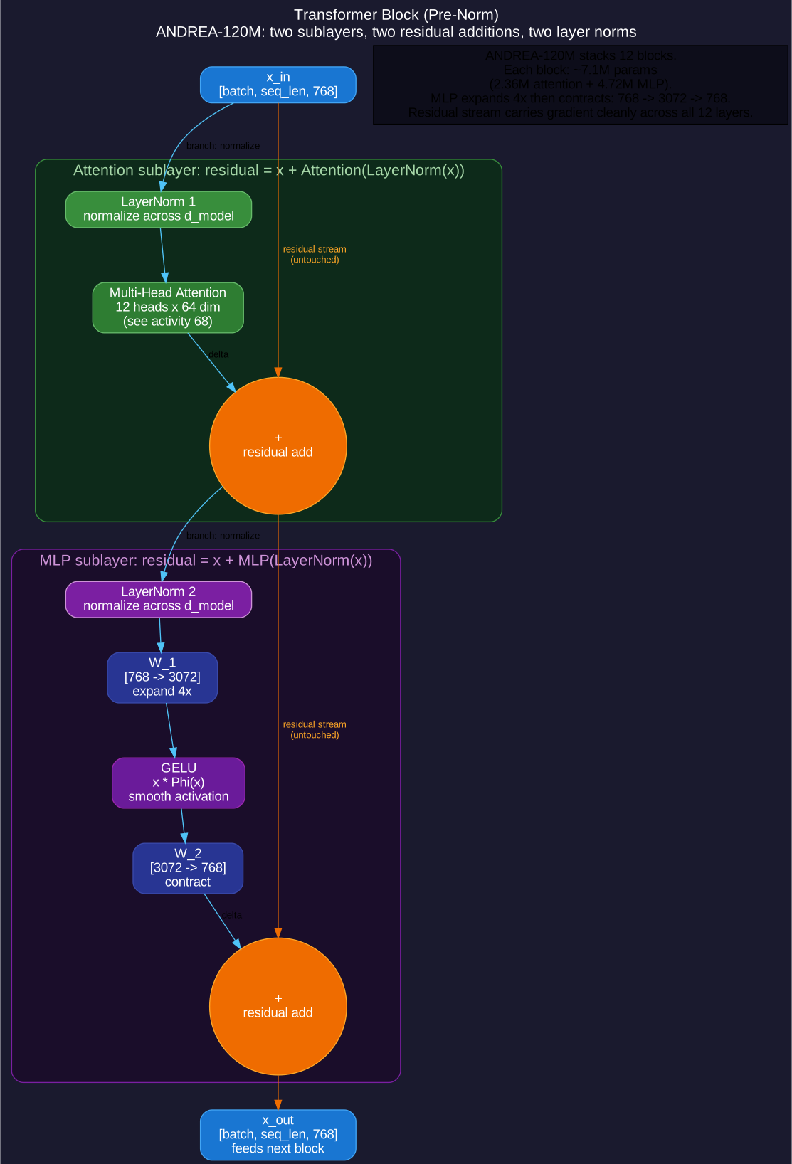
Two Sublayers
A transformer block contains exactly two sublayers, each operating on a token sequence of shape [batch, seq_len, d_model]:
1. Multi-head attention sublayer. Tokens look at each other. Activity 68 covered this in detail. Output shape matches input shape.
2. Feed-forward MLP sublayer. Each token transforms independently through a two-layer perceptron. No cross-token information flow. Output shape matches input shape.
Both sublayers preserve the [batch, seq_len, d_model] shape. That preservation lets blocks stack: layer N's output feeds layer N+1's input with no shape acrobatics.
What Each Sublayer Contributes
Attention moves information across positions: a token at position 17 can pull information from positions 1 through 16. The MLP transforms information within each position: a token's representation gets reshaped through learned non-linear functions, but never sees its neighbors.
Stacking blocks alternates these two operations. Layer 1 attention mixes positions. Layer 1 MLP reshapes per-position. Layer 2 attention mixes again, now over the reshaped representations. This alternation grows expressive power with depth.
ANDREA's Stack
| Variant | n_layer | n_head | d_model | mlp_dim |
|---|---|---|---|---|
| ANDREA-12M | 6 | 12 | 384 | 1536 |
| ANDREA-120M | 12 | 12 | 768 | 3072 |
| ANDREA-480M | 16 | 24 | 1536 | 6144 |
Notice mlp_dim = 4 × d_model across the family. That ratio holds in nearly every modern transformer. Section 3 walks through why.
Naming The Sublayers
Why Skip Connections Matter
The Residual Pattern
Each sublayer wraps its computation in a residual connection. The output adds back the input:
x = x + Attention(LayerNorm(x))     # attention sublayer
x = x + MLP(LayerNorm(x))           # MLP sublayer
Inside each sublayer, the function Attention(...) or MLP(...) produces a delta. The block does not replace the input; it adds a learned correction.
Why This Matters
Three reasons residual connections dominate deep architectures:
1. Gradient flow. During backpropagation, the addition gives gradients a direct path from output back to input, bypassing the sublayer. A 12-layer stack without residuals would lose gradient signal long before reaching the embeddings; with residuals, gradient magnitude stays usable through hundreds of layers.
2. Identity initialization. At initialization, sublayer weights produce small outputs. The residual connection means layer N initially passes through nearly unchanged. Training learns deltas progressively from a working starting point.
3. Compositional learning. Each block learns a refinement, not a replacement. Layer 1 might add positional information. Layer 2 might add syntactic structure. Layer 7 might add semantic relationships. The residual stream accumulates.
Layer Normalization
Before each sublayer, LayerNorm rescales each token's representation to zero mean & unit variance, then applies learned per-feature gain & bias:
y = gamma * (x - mean(x)) / sqrt(var(x) + epsilon) + betaMean & variance get computed across the d_model dimension, separately for every token. Two learned vectors (gamma, beta, each shape [d_model]) restore expressive scale. Normalization keeps activations in a numerically stable range; without it, small training instabilities snowball into NaN gradients.
Pre-Norm vs Post-Norm
A Subtle But Critical Choice
Two ways to wire layer norm into a residual sublayer:
Post-norm (original 2017 paper):
x = LayerNorm(x + Attention(x))Layer norm sits after the residual addition. The residual stream itself gets normalized at every layer.
Pre-norm (modern standard, used in ANDREA):
x = x + Attention(LayerNorm(x))Layer norm sits before the sublayer, inside the residual branch. The residual stream stays un-normalized; only the input to the sublayer gets rescaled.
Why Pre-Norm Won
Post-norm trains poorly without LR warmup & careful hyperparameter tuning. Gradients explode in early layers because each layer norm scrambles the residual stream's accumulated state. The original 2017 paper used post-norm with extensive tuning; subsequent work (GPT-2, LLaMA, ANDREA) standardized on pre-norm.
Pre-norm trains stably. The residual stream accumulates clean across all layers; only sublayer inputs get normalized for numerical stability. Modern transformers default to pre-norm, & ANDREA inherits that choice.
Final Block Equation
Combining residuals, layer norm in pre-norm position, & both sublayers gives ANDREA's full block:
def block_forward(x):
    x = x + Attention(LayerNorm(x))   # attention sublayer
    x = x + MLP(LayerNorm(x))         # MLP sublayer
    return x
Two sublayers, two residual additions, two layer norms (note: each sublayer has its own layer norm; ANDREA-120M has 24 layer norms across 12 blocks plus a final one at output, so 25 total). Repeat 12 times. That's the trunk of ANDREA-120M.
Why Pre-Norm Stabilizes Training
Two Linear Layers, One Activation
Three Operations
The MLP sublayer is a two-layer perceptron with a non-linear activation between the layers:
def mlp_forward(x):
    h = x · W_1 + b_1        # expand: d_model → mlp_dim
    h = GELU(h)              # non-linear activation
    y = h · W_2 + b_2        # contract: mlp_dim → d_model
    return y
Three operations. Two linear, one non-linear. The first linear expands width; the second contracts back.
The 4× Expansion Ratio
Modern transformers set mlp_dim = 4 × d_model. ANDREA-120M:
d_model = 768
mlp_dim = 4 × 768 = 3072
W_1 shape = [768, 3072]      # ~2.36M params
W_2 shape = [3072, 768]      # ~2.36M params
MLP params per block = 4.72M (ignoring biases)
Two MLPs sit between every pair of attention sublayers (one per block). Twelve blocks × 4.72M ≈ 56.6M MLP parameters total in ANDREA-120M, roughly half of all parameters.
Why 4×
The 4× ratio emerged empirically. Smaller ratios reduce model capacity. Larger ratios produce diminishing returns per parameter spent. Across decades of architecture search, 4× has held up; it appears in GPT, BERT, T5, LLaMA, & ANDREA.
Recent work (PaLM, Chinchilla) found that gating mechanisms (SwiGLU) can use 8/3× expansion with comparable capacity at less cost; ANDREA stays with classic GELU + 4× for simplicity.
GELU: A Smooth Activation
What GELU Computes
GELU (Gaussian Error Linear Unit) is the standard activation between MLP layers in modern transformers. Its formula:
GELU(x) = x · Φ(x)Φ(x) is the cumulative distribution function of the standard normal: the probability that a standard Gaussian random variable falls at or below x. Computed numerically:
Φ(x) ≈ 0.5 × (1 + tanh(sqrt(2/π) × (x + 0.044715 × x³)))Behavior By Region
- For large positive x: Φ(x) ≈ 1, so GELU(x) ≈ x. Like ReLU.
- For large negative x: Φ(x) ≈ 0, so GELU(x) ≈ 0. Like ReLU.
- Near x = 0: Φ(x) ≈ 0.5, so GELU(0) = 0 exactly. Smooth transition through the origin.
Unlike ReLU, GELU lets some negative inputs through, weighted by Φ(x). A small negative input still contributes a small negative output, just less than the full input would.
Why GELU Outperformed ReLU
Empirically, transformers trained with GELU reach lower loss than transformers trained with ReLU at the same parameter count. The smoothness around zero matters: ReLU's hard cutoff at zero produces gradient discontinuities; GELU's smooth curve provides cleaner gradients for backpropagation.
ANDREA's training engine microgpt_cuda.cu ships a hand-written GELU CUDA kernel. The kernel uses the tanh approximation above; modern GPUs include tanh as a single-instruction op.
Computing MLP Parameters
Twelve Blocks Compose Into ANDREA-120M
From Block to Model
ANDREA-120M's full forward pass:
def model_forward(token_ids):
    x = token_embed(token_ids) + position_embed(positions)
    for block_idx in range(n_layer):       # 12 blocks
        x = block_forward(x)               # attention + MLP w/ residuals
    x = LayerNorm(x)                       # final norm
    logits = x · token_embed.T             # tied weights for output projection
    return logits
Six lines. The bulk lives inside block_forward, called twelve times. Embeddings start the pipeline; tied unembedding (the same matrix used for input lookup, transposed for output projection) ends it.
Depth As Composition
Each block reads the residual stream, computes a delta, & adds it back. After twelve passes, the stream contains accumulated contributions from every block. Internally, layers tend to specialize:
- Early layers (1-3): syntactic patterns, positional structure
- Middle layers (4-8): word relationships, phrase boundaries
- Late layers (9-12): semantic content, factual recall
This specialization emerges from training pressure, not from architectural choices. The same uniform block design produces specialized layers when trained on language.
Total Block Parameters
| Component | Per block | Across 12 blocks |
|---|---|---|
| Attention projections (4×W) | 2.36M | 28.3M |
| MLP weights (W_1 + W_2) | 4.72M | 56.6M |
| Layer norms (gamma, beta) | ~3K (negligible) | ~37K |
| Total per block | ~7.1M | ~85M |
85M parameters in the trunk. Add ~13M in token embeddings (8449 vocab × 768 d_model × 2 for tied input/output) plus a final layer norm, & ANDREA-120M's parameter count lands at roughly 120M. The block design accounts for two-thirds; embeddings the rest.