Query, Key, Value
Three Linear Maps from a Same Input
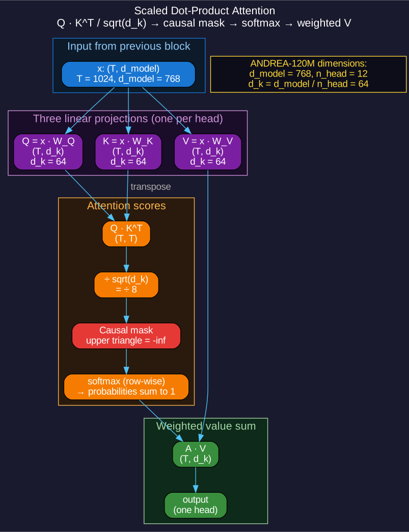
After embedding (activity 4), each position carries a 768-dimensional vector x_t. Attention starts by producing three distinct projections of x:
Q (query): what does this position want to know?
K (key): what does this position offer to other positions?
V (value): what content does this position deliver if attended to?
Each projection comes from a learned weight matrix:
Q = x · W_Q     # W_Q shape: (d_model, d_k)
K = x · W_K     # W_K shape: (d_model, d_k)
V = x · W_V     # W_V shape: (d_model, d_k)
Three matrices, all trained via backpropagation. A model learns: at this position, what query best retrieves useful past context? What key advertises this position's content well? What value delivers if selected?
A Library Analogy
Imagine a library card catalog. You walk in with a topic in mind (your query). Every card lists keywords (a key). When your topic matches a card's keywords, you grab a book contents (a value). Attention does this for every token in parallel: every position queries every other position, ranks alignment, & retrieves a weighted combination of value vectors.
ANDREA-120M Dimensions
| Quantity | Value | Notes |
|---|---|---|
| d_model | 768 | Vector size at every position |
| n_head | 12 | Parallel attention heads |
| d_k | 64 | Per-head dim (= d_model / n_head) |
| T | 1024 | Context length |
d_k = d_model / n_head = 768 / 12 = 64. Each head sees a 64-dimensional slice of a full 768-dimensional space. Activity 6 (grow_a_language_model_multi_head) covers a per-head split in detail.
Compute d_k
Why Divide by sqrt(d_k)
A Score Matrix
Once Q & K exist (each shape (T, d_k)), attention computes a score matrix:
scores = Q · K^T # shape: (T, T)scores[i, j] = how strongly position i's query aligns with position j's key. Every (i, j) pair gets one score: 1024 × 1024 = 1,048,576 scores per attention head per forward pass.
Why Divide
Dot products of two random d-dimensional unit vectors have magnitude on order of sqrt(d). Without scaling, scores grow with d_k:
- d_k = 64: typical dot products on order of 8.
- d_k = 256: typical dot products on order of 16.
- d_k = 4096: typical dot products on order of 64.
Big scores produce a peaky softmax (one position dominates, gradients vanish elsewhere). Training stalls. Scaling fixes a magnitude:
scaled_scores = (Q · K^T) / sqrt(d_k)For ANDREA-120M, sqrt(d_k) = sqrt(64) = 8. Every score gets divided by 8. Magnitudes stay roughly unit-scale regardless of d_k. Softmax stays well-behaved. Gradients flow.
Vaswani's Original Justification
From Attention Is All You Need (2017): 'For large values of d_k, the dot products grow large in magnitude, pushing the softmax function into regions where it has extremely small gradients.' A sqrt(d_k) divisor counteracts that growth.
A Code View
Inside microgpt_cuda.cu, this scaling appears as a literal division:
scores[i][j] = dot(Q[i], K[j]) * (1.0f / sqrtf(d_k));One float multiplication per score. Cheap. Critical.
Scale at d_model = 4096
Why Position i Cannot See Position j > i
A Constraint Born from Generation
ANDREA generates one token at a time. At inference, position 0 produces a first token, then position 1 sees position 0's output & produces a second token, & so on. A model never has access to future tokens during generation.
Training must mirror this. If during training position 5 could attend to position 6, a model would learn a shortcut: 'predict token 6 by reading token 6'. At inference, that shortcut disappears (token 6 doesn't exist yet). A model's training-versus-inference behavior would diverge catastrophically.
A Mask
A causal mask blocks attention from any position i to any position j > i. Implementation: set scaled_scores[i][j] = -infinity wherever j > i. After softmax, those entries become exp(-inf) = 0. Mask zeros out attention to future positions cleanly.
for i in range(T):
    for j in range(T):
        if j > i:
            scaled_scores[i][j] = -1e9   # effectively -inf
After softmax (row-wise), each row sums to 1, but only entries [0, i] carry probability mass. Position i mixes information only from past positions.
Visualizing a Mask
A score matrix shape (T, T) with mask applied looks like a lower-triangular structure:
scaled_scores after mask, row-wise softmax:

row 0:  [1.0, 0,   0,   0,   ...]   # sees only itself
row 1:  [0.4, 0.6, 0,   0,   ...]   # sees positions 0, 1
row 2:  [0.2, 0.3, 0.5, 0,   ...]   # sees 0, 1, 2
row 3:  [0.1, 0.2, 0.3, 0.4, ...]   # sees 0, 1, 2, 3
...
Strict lower-triangular probability distribution per row. Future stays invisible.
Why a Decoder-Only Transformer Needs This
Decoder-only models like ANDREA, GPT, & LLaMA all share one objective: predict next token from past. A causal mask makes that objective trainable in parallel: every position computes its own next-token prediction at once, & no position cheats by peeking ahead.
Mask & Flavor
From Scores to Output
Softmax: Scores to Probabilities
Masked, scaled scores still range over real numbers. Softmax converts each row into a probability distribution:
A[i][j] = exp(scaled_scores[i][j]) / sum_k exp(scaled_scores[i][k])Three properties result:
- A[i][j] >= 0 for all (i, j).
- sum_j A[i][j] = 1 for every row i.
- Larger raw scores produce larger probabilities (monotone).
Row i's probability vector tells a model: how much should position i attend to each prior position when computing its output?
Weighted V Sum
A final attention output for position i:
output[i] = sum_j A[i][j] · V[j]Each value vector V[j] gets weighted by attention probability A[i][j], then summed. Position i's output combines value vectors from every prior position, weighted by relevance.
In matrix form, all positions at once:
Attention(Q, K, V) = softmax(mask(Q · K^T / sqrt(d_k))) · VOne line. A whole attention mechanism. Vaswani et al. wrote that line in 2017; transformers haven't fundamentally changed since.
Per-Head Output Shape
Output of one attention head: shape (T, d_k). For ANDREA-120M: (1024, 64). All 12 heads compute in parallel; their outputs concatenate to (1024, 768) & feed into a final linear projection (W_O), then on to a transformer block's MLP.
Activity 6 (grow_a_language_model_multi_head) covers a multi-head split. Activity 7 (grow_a_language_model_transformer_block) covers everything that surrounds attention: residual connections, layer norm, MLP.