PAC as a Two-Axis Plane
Two Axes, One Sample-Count Surface
Plot ε on horizontal axis (error tolerance, range 0 to 1). Plot δ on vertical axis (probability of failure, range 0 to 1). Each point in this unit square corresponds to a (ε, δ) demand pair.
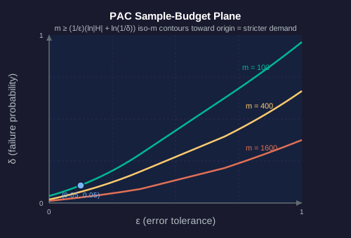
Above each point sits a sample-count value m(ε, δ) = (1/ε)(ln|H| + ln(1/δ)). Together, those m values trace a curved surface above our square. Stricter demands (smaller ε, smaller δ) pull our surface upward; looser demands flatten it.
Iso-Sample Contour Lines
Project our surface back down to our plane as iso-m contours. Every (ε, δ) pair on a single contour requires our same sample budget. Move along a contour to trade error tolerance for confidence at fixed cost.
Halving an Axis
Halving ε along our horizontal moves m up by factor 2 (linear in 1/ε). Halving δ along our vertical moves m up by ln(2) ≈ 0.69 (logarithmic in 1/δ). Geometry tells us: error tolerance carries a steeper cost than confidence.
Reading the Budget Surface
We sit at point (ε = 0.05, δ = 0.05) for hypothesis class |H| = 10⁶. Sample requirement m₀ = (1/0.05)(ln(10⁶) + ln(20)) = 20 × (13.8 + 3.0) = 336.
Dichotomies on Point Clouds
What Shattering Looks Like
Place n points in our plane. Pick a hypothesis class (linear classifiers = straight lines). Count how many distinct ways our class can label those n points (+/− on each side of a line). Call this count Π_H(n).

If Π_H(n) = 2ⁿ, our class shatters that point set — it can produce every possible labeling. If Π_H(n) < 2ⁿ, some labelings cannot occur.
Three Points in General Position
Linear classifiers in ℝ² shatter any 3 non-collinear points. 2³ = 8 labelings; all 8 achievable by some line. Pick any 3 points; for each ±/± labeling, draw a line that separates positives from negatives.
Four Points Refuse to Shatter
Place 4 points at corners of a square. Try to label diagonal pair as positive & anti-diagonal pair as negative (XOR labeling). No straight line separates them. So Π_H(4) ≤ 14 < 16 = 2⁴.
VC Dimension as Maximum Shatter Size
VC(linear ℝ²) = 3. We can shatter 3 points; we cannot shatter 4. VC counts maximum dichotomy capacity of our hypothesis class.
Geometric Intuition
Higher VC = our class draws more elaborate decision boundaries. Linear (VC = d+1 in d dimensions) draws hyperplanes. Polynomials draw curves. Neural networks draw highly folded manifolds. More foldability = more dichotomies = higher VC = higher sample requirement.
Counting Dichotomies
Consider linear classifiers in ℝ² (lines). We have 5 points placed in general position (no 3 collinear, none redundant).
Probability Mass on Hypothesis Manifold
Picturing PAC-Bayes
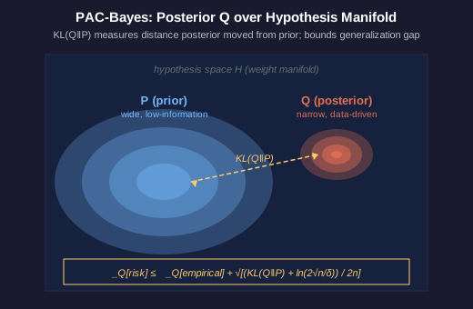
Picture our hypothesis space as a high-dimensional manifold. Each point on this manifold corresponds to one weight configuration of a neural network. Prior P assigns a probability distribution across our manifold (often Gaussian centered at initialization). Posterior Q concentrates probability mass where training data drove our weights.
KL Divergence as Geometric Distance
KL(Q‖P) measures how far Q drifted from P. Geometric reading: how much our posterior cloud moved from prior cloud, weighted by how unlikely each posterior region was under our prior.
Small KL = Q overlaps P heavily. Posterior barely moved. Generalization gap stays small.
Large KL = Q concentrated in regions P assigned little mass to. Posterior moved a lot. Generalization gap grows.
Why This Geometry Matters
Imagine SGD as a search trajectory across our hypothesis manifold. Trajectory ends at a basin of low training loss. PAC-Bayes asks: how wide is this basin?
Wide basin = many neighboring weight configurations also achieve low training loss. Posterior Q can spread over a wide region & still have low risk. KL(Q‖P) stays bounded. Generalization gap small.
Narrow basin = only a thin set of weights achieves low loss. Posterior must concentrate sharply. KL grows. Generalization gap widens.
This connects directly to flat-vs-sharp minima discourse (Hochreiter & Schmidhuber 1997, Keskar et al 2017). Flat minima generalize better because they support wider posteriors with smaller KL.
Reading a Basin Width
Two trained models reach identical training loss but live in different basins:
- Model A: flat basin, posterior spreads over region with KL(Q_A‖P) = 50 nats.
- Model B: sharp basin, posterior concentrates with KL(Q_B‖P) = 500 nats.
Both trained on n = 10,000 examples with empirical risk 0.05, δ = 0.05.
A Curve That Falls Where Theory Predicted Rise
Classical U-Curve
Plot model capacity on horizontal axis. Plot test risk on vertical axis. Classical bias-variance theory predicts:
- Low capacity: high bias, high test risk (underfit)
- Mid capacity: low bias + low variance, low test risk (sweet spot)
- High capacity: low bias, high variance, high test risk (overfit)
Result: U-shaped curve. Pick capacity at our bottom.
What Belkin et al (2019) Observed
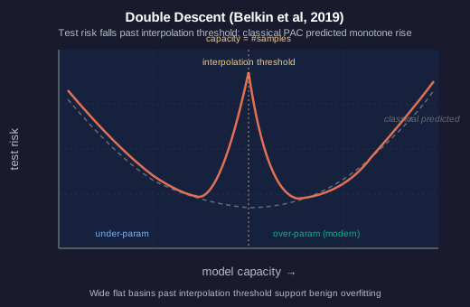
Past interpolation threshold (capacity where model exactly fits training data with zero error), test risk DROPS again. Curve reads: descent → peak at interpolation → second descent. Two descents, one curve.
Geometric Reading of Second Descent
At interpolation threshold, model has just enough capacity to fit training data — only one (or few) interpolating solutions exist & they tend to be jagged. Generalization suffers because solution chosen is forced.
Past interpolation threshold, MANY interpolating solutions exist. SGD has freedom to pick a smooth one (minimum-norm, low-curvature). Geometric picture: solution manifold becomes wider & flatter. SGD's implicit regularization picks benign solutions from this flat manifold. Test risk falls.
Why Classical Theory Misses This
VC dimension counts solution-set capacity but ignores which solution gets chosen. Classical bound assumes worst-case empirical risk minimizer. Reality: SGD reliably picks our flattest, smoothest interpolating solution. Once we count SOLVER-CHOSEN solutions instead of all solutions, second descent makes sense.
Geometric Take-Home
Capacity matters less than basin geometry. Wide flat basins (post-interpolation) generalize better than narrow sharp ones (at interpolation). Modern theory tries to bound generalization by basin width, not by parameter count.
Locating the Two Descents
On a double descent curve, three regions matter: (1) under-parameterized regime, (2) interpolation peak, (3) over-parameterized regime.
Power-Law Surface in Parameter-Token Space
A 3D Surface
Plot parameters N on one horizontal axis. Plot tokens D on a second horizontal axis. Plot loss L on vertical. Empirical loss carves a power-law surface across this (N, D) plane:
L(N, D) ≈ (Nc/N)^αN + (Dc/D)^αD + L∞
Surface slopes downward as either N or D grows. Slopes follow log-linear power laws (straight lines in log-log plot). Asymptote L∞ stays positive — irreducible loss our model cannot shrink past.
Compute-Optimal Ridge
Fix total compute budget C ∝ N × D (parameters × tokens, roughly). Slice our surface along this constraint. Slice trace cuts a 2D curve through 3D surface. Bottom of this curve = compute-optimal point.
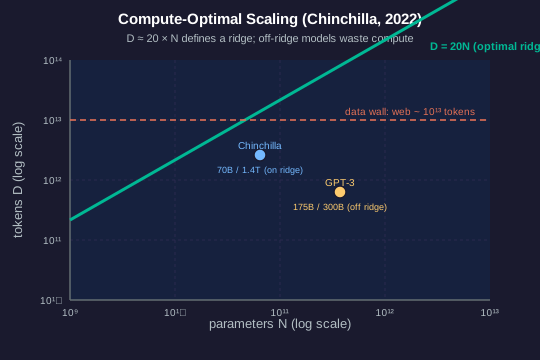
Chinchilla (Hoffmann et al 2022) computed this bottom analytically: D_opt ≈ 20 × N. Curve along compute budget = a ridge. Walking along ridge: equal compute, decreasing loss. Walking off ridge (more parameters than 20× tokens, or fewer): wasted compute.
Geometric Reading of GPT-3 vs Chinchilla
GPT-3: 175B params, 300B tokens. Chinchilla-optimal would want 175B × 20 = 3500B tokens. GPT-3 sits far off the compute-optimal ridge in our parameter-heavy direction. Chinchilla itself: 70B params trained on 1400B tokens. 1400 / 70 = 20 — exactly on ridge. Chinchilla beat GPT-3 with less than half its parameter count by sitting on geometric optimum.
Data Wall as Vertical Plane
Public web ~10¹³ usable tokens. This plots as a vertical wall at D = 10¹³ on our parameter-token plane. Beyond this wall, compute-optimal training requires N ≤ D / 20 = 5 × 10¹¹ params. Walls beyond N = 5 × 10¹¹ either run under-trained (off-ridge) or require synthetic / multimodal / RL data to push wall outward.
Walking the Compute-Optimal Ridge
We sit at GPT-3 coordinates: N = 175B params, D = 300B tokens. Compute proxy C = N × D = 5.25 × 10²² param-tokens.
Beta Posterior Tightening into a Needle
A Probability Density on [0, 1]
Beta(α, β) is a probability density over the unit interval [0, 1]. Variable: ε = true error rate. Shape: α controls mass on high-ε side; β controls mass on low-ε side.
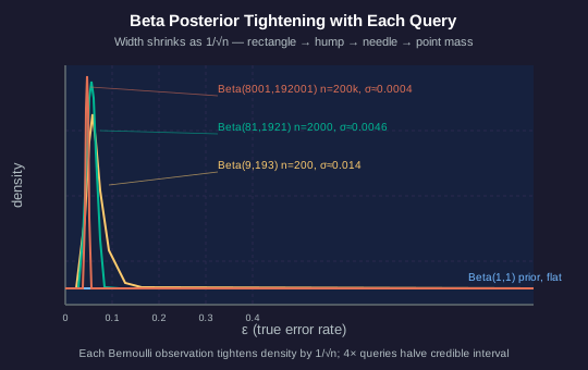
Beta(1, 1): uniform — no information, flat density across [0, 1].
Beta(α, β) with α + β large: concentrated peak at α / (α + β).
Width of Beta peak shrinks as 1/√(α+β). Adding 100 observations to our prior tightens the peak by factor √100 = 10. Adding 10000 observations tightens by √10000 = 100.
Geometric Reading of an Audit Run
Start: Beta(1, 1) = flat rectangle on [0, 1]. Maximum uncertainty about ε.
After 200 queries with 8 falsifications: Beta(9, 193). Mean = 9/202 ≈ 0.045. Density now a sharp hump centered near 0.045 with characteristic width σ ≈ 0.014.
After 2000 queries with 80 falsifications: Beta(81, 1921). Mean still ≈ 0.045, but width σ ≈ 0.0046. Hump three times sharper.
After 200,000 queries with 8000 falsifications: Beta(8001, 192,001). Mean ≈ 0.040, width σ ≈ 0.0004. Hump becomes a needle.
Geometric Convergence to a Point Mass
As n → ∞, Beta posterior collapses to a Dirac delta at true ε. Geometry: rectangle → wide hump → narrow hump → needle → point. Each query tightens our distribution by 1/√n.
Why This Beats Theoretical PAC Bounds
Theoretical PAC bounds give a STATIC ε estimate based on hypothesis class size. Beta posterior gives a DYNAMIC ε estimate that tightens with every observation, calibrated against your real-world distribution. Theoretical bound = a guarantee under worst-case assumptions. Empirical audit = a measurement of actual reality.
How Many Queries to Halve the Credible Interval?
We currently sit at Beta(9, 193) after 200 queries: mean ε ≈ 0.045, σ ≈ 0.014. We want to halve the credible-interval width to σ ≈ 0.007.